Each type of learning process of a neural network model is usually summarized as a training algorithm. There are many algorithms for training, and their characteristics and performance are different.

The abstraction of the problem transforms the learning process of the neural network into the minimum problem of the loss function f. In general, the loss function consists of an error term and a regular term. The error term measures the degree of fitting of the neural network model on the training data set, while the regular term measures the complexity of the model to prevent overfitting.
The function value of the loss function is determined by the parameters of the model (weight value and offset value). We can combine the two parts of the parameters into an n-dimensional weight vector, denoted as w. The figure below is a graphical representation of the loss function f(w).
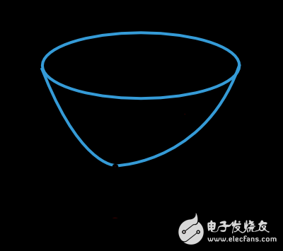
As shown in the figure above, w* is the minimum value of the loss function. By arbitrarily selecting a point A in space, we can calculate the first-order and second-order derivatives of the loss function. The first derivative can be expressed as a vector:
áif(w) = df/dwi (i = 1,...,n)
Similarly, the second derivative of the loss function can be expressed as a Hessian Matrix:
Hi,jf(w) = d2f/dwi·dwj (i,j = 1,...,n)
The problem of solving multivariable continuous differentiable functions has been widely studied. Many traditional methods can be directly applied to the solution of neural network models.
One-Dimensional Optimization Method Although the value of the loss function needs to be determined by multiple parameters, the one-dimensional optimization method is also very important here. These methods are often used to train neural network models.
Many training algorithms first calculate a training direction d, and a rate η to represent the change in the loss value in this direction, f(η). The next image shows this one-dimensional function.
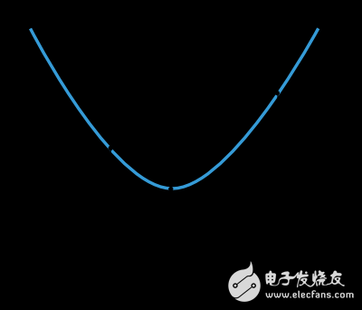
f and η* are within the interval in which η1 and η2 are located.
Thus, the one-dimensional optimization method is to find the minimum value of a given one-dimensional function. The golden segmentation method and the Brent method are two widely used algorithms. These two algorithms continually reduce the range of the minimum until the distance between the two points η1 and η2 is less than the set threshold.
Multidimensional optimization method We abstract the learning problem of neural network into the problem of finding the parameter vector w*, so that the loss function f takes the minimum value at this point. Suppose we find the minimum point of the loss function, then we think that the gradient of the neural network function here is equal to zero.
Usually, the loss function is a nonlinear function, and it is difficult to accurately obtain the optimal solution using the training algorithm. Therefore, we try to search through the parameter space step by step to find the optimal solution. At each search step, the parameters of the neural network model are recalculated and the loss values ​​are correspondingly reduced.
We first randomly initialize a set of model parameters. Then, each time the iteration updates the set of parameters, the loss function value also decreases. When a particular condition or termination condition is met, the entire training process ends.
Now let's introduce the most important training algorithms for several neural networks.

The gradient descent method is the simplest training algorithm. It only needs the information of the gradient vector, so it belongs to the first-order algorithm.
We define f(wi) = fiand áf(wi) = gi. The algorithm starts at W0 and then moves from wi to wi+1 along the di=-gi direction in step i, iterating over and over until the termination condition is met. The iterative formula of the gradient descent algorithm is:
Wi+1 = wi- di·ηi, i=0,1,...
The parameter η is the learning rate. This parameter can be set to a fixed value or a one-dimensional optimization method to gradually update the calculation along the direction of the training. People generally tend to gradually update the computational learning rate, but many software and tools still use a fixed learning rate.
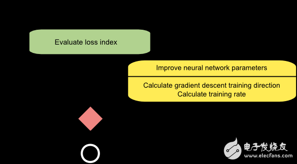
The figure below is a flow chart of the gradient descent training method. As shown in the figure, the parameter update is divided into two steps: the first step calculates the direction of the gradient drop, and the second step calculates the appropriate learning rate.
The gradient descent method has a serious drawback. If the gradient of the function exhibits a slender structure as shown, the method requires many iterations. Moreover, although the direction of the gradient drop is the direction in which the loss function value decreases the fastest, this is not necessarily the fastest path. The figure below depicts this issue.
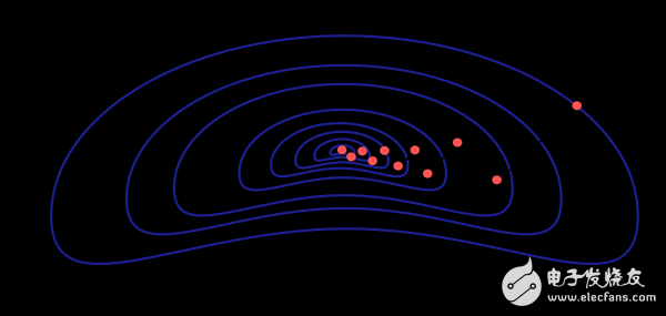
When the neural network model is very large and contains thousands of parameters, the gradient descent method is our recommended algorithm. Because this method only needs to store the gradient vector (n space) without storing the Hessian matrix (n2 space)
The JUK universal Screw Terminal Block series has the typical features which are decisive for practical applications:
l The universal foot allows the terminal blocks to be easily snapped onto the NS35 or NS32 DIN Rail with G shape.
l Closed screw guide holes ensure screwdriver operation perfect.
l For terminal block with different wire cross-sectional areas, complete accessories are available, such as end plates, partition plates, etc.
l Potential distribution achieved by fixed bridges in the terminal center or insertion bridges in the clamping space.
l Same shape and pitch Grounding Terminal Blocks as the JUK universal series.
l Adopt ZB marker strip system,achieve unified identification.
Cable Terminal Connectors,90 Degree Spade Terminal Connector,Insulated Spade Terminal,2 Pin Terminal Connector
Wonke Electric CO.,Ltd. , https://www.wkdq-electric.com